A common task in machine learning is to estimate or optimize “log-sum-exp” functions with (potentially continuously) many terms such as $$ \log \Big( \int_{\mathcal{X}} e^{v(x)} dq(x) \Big),$$ where \(v: \mathcal{X} \to \mathbb{R}\) is some potential function, and \(q\) is a probability distribution on the set \(\mathcal{X}\). This has many applications throughout data science, often through the normalization of probabilistic models, but also as a smooth approximation to the maximum, in transformers through its derivatives, or in reinforcement learning when using entropy regularization [19]. Sometimes the set \(\mathcal{X}\) is finite (potentially big) and the integral can be done by explicit summing, but often an exact computation is infeasible, and sampling from the probability distribution \(q\) is used instead.
The key difficulty comes from the variance of such estimates, in particular when \(v\) takes large values. In the simplest example, for \(z_1,\dots,z_n \in \mathbb{R}\) independent and normally distributed with mean \(\mu\) and variance \(\sigma^2\), the relative squared error for estimating \(\mathbb{E}[e^z]\) is $$\frac{ {\rm var}\big( \frac{1}{n} \sum_{i=1}^n e^{z_i} \big) }{( \mathbb{E}[ e^{z} ])^2} = \frac{1}{n} \frac{ {\rm var}(e^z) }{( \mathbb{E}[ e^{z} ])^2} = \frac{ e^{\sigma^2}-1}{n}.$$ It converges to zero when \(n\) grows (as can be expected from the law of large numbers), but explodes exponentially when \(\sigma\) grows. Even taking the logarithm does not change the exploding variance, that is, \({\rm var}\big( \log \big( \frac{1}{n} \sum_{i=1}^n e^{z_i} \big)\big)\) also can be shown to grow asymptotically similarly in \(\frac{ e^{\sigma^2}-1}{n}\) (when \(n\) is large, as can be obtained from the delta method).
While difficult to estimate, the log-sum-exp function comes with many nice properties (and that’s why people love it); I particularly like the fact that (1) it is a smooth approximation to the maximum (see, e.g., this earlier post), and (2) it is a way to normalize probabilistic models that is adapted to maximum likelihood estimation, in particular in hierarchical probabilistic models, where (conditional) independence assumptions lead to separability of associated loss functions (as thoroughly used in probabilistic graphical models).
The main question I try to answer in this post is:
Can we keep the advantages of optimizing log-sum-exp functions while being less exposed to their computational / statistical disadvantages?
The magic of least-squares
At the other end of the spectrum sits least-squares regression, with essentially the exact opposite features:
- On the positive side, we obtain computational and statistical simplicity in various forms, e.g., it leads to closed-form estimation for linear models through linear algebra, it is based on computing moments with fixed controlled variance, and it leads to sharp analyses in various setups (acceleration, stochastic gradient descent, etc.). See, e.g., this post on acceleration, and this one on averaging.
- On the negative side, using least-squares regression for all prediction problems, particularly with discrete outputs, creates some artefacts. The traditional example is classification with Gaussian class-conditional data (with identical covariance matrices), where least-squares on the one-hot encoded outputs has problems, such as “masking” (see [13, Section 2.4] and the example below), or high approximation error compared with using multinomial logistic regression (a.k.a. softmax regression), because then the log conditional probabilities are affine.
Can we reconcile them? In other words, is least-squares really all I need? (my colleagues sometimes mock me for my love of least-squares).
Note that there is another (classic) attempt at seeing the world through least-squares: doing it in series through Newton’s method, leading in this context to iteratively reweighted least-squares, but this is for computations only, with no statistical improvement. What we are aiming at is stronger: can we get least-squares-based closed-form estimators for maximum-likelihood problems that typically require optimization of a convex function (such as logistic or softmax regression)?
Interestingly, my new attempt can be summarized in one integral equation $$ t \log t\, – t + 1 = \int_0^1 \!\! \frac{ (t-1)^2}{\rho t + 1-\rho} (1-\rho) d\rho,$$ which can be checked by usual integration tricks. Let’s see why and how!
Relative density estimation as a testbed
In this post, I look at a simple fundamental problem where we can study and compare various estimation frameworks, noting that it can be extended in several ways (in particular, through mutual information, see below).
We consider two probability distributions \(p\) and \(q\) on \(\mathcal{X}\); our goal is to estimate the logarithm of the relative density \(\log \big(\frac{dp}{dq}(x)\big)\). This turns out to be equivalent to estimating the Kullback-Leibler (KL) divergence because of the variational formulation [1] $${\rm KL}(p\|q) = \int_{\mathcal{X}} \log \big(\frac{dp}{dq}(x)\big) dp(x) = \sup_{v: \mathcal{X} \to \mathbb{R}} \int_{\mathcal{X}} v(x) dp(x) + 1\, – \int_{\mathcal{X}} e^{v(x)} dq(x). \tag{1} $$
This is one particularly important instance of an \(f\)-divergence (see, e.g., [2]), with the following definition and variational formulation based on the Fenchel conjugate \(f^\ast\) of \(f\): $$D(p\|q) = \int_{\mathcal{X}} f \big( \frac{dp}{dq}(x) \big) dq(x)= \sup_{v: \mathcal{X} \to \mathbb{R}} \int_{\mathcal{X}} v(x) dp(x) \, – \int_{\mathcal{X}} f^\ast(v(x)) dq(x),$$ the representation being a consequence of \(f(t) = \sup_{ u \in \mathbb{R}} ut-f^\ast(u)\) applied to each \(t = \frac{dp}{dq}(x)\). The KL divergence corresponds to \(f(t) = t \log t \, – t + 1\) and \(f^\ast(u) = e^u \, – 1\).
Note that for the particular case of the KL divergence, when optimizing with respect to a constant on top of \(v\), we obtain the Donsker-Varadhan representation [3] $${\rm KL}(p\|q) = \sup_{v: \mathcal{X} \to \mathbb{R}} \int_{\mathcal{X}} v(x) dp(x)\, – \log \Big( \int_{\mathcal{X}} e^{v(x)} dq(x) \Big). \tag{2}$$
We see the log-sum-exp function appearing explicitly. To estimate the potential \(v\) from i.i.d. samples from \(p\) and \(q\), the traditional variational approach corresponds to replacing integrals with empirical averages. For \(q\), this leads to a potentially unstable empirical average when only samples are available. The goal of this post is to explore another way (I present the main principles behind this new framework; see [7] for more details).
The framing through \(f\)-divergences is really key to the new approach, as other divergences will be instrumental in the definition. Before we move on, we state another (equivalent) variational formulation with two potentials \(v\) and \(w\), which we will need later: \(D(p\|q)\) is equal to $$\sup_{v,w: \mathcal{X} \to \mathbb{R}} \int_{\mathcal{X}} v(x) dp(x) + \int_{\mathcal{X}} w(x) dq(x) \mbox{ such that } \forall x \in \mathcal{X}, w(x) \leqslant -f^\ast(v(x)). \quad \tag{3}$$ At optimum, we get \(w(x) = -f^\ast(v(x))\), and we recover Eq. (1) in the KL case. The constraint is convex, but for \(f(t) = t \log t – t + 1\), it is far from what traditional convex optimization methods typically allow. This formulation appears in [25, Theorem 4.4] and has the nice property of preserving the symmetry of the problem (that is, if \(p\) and \(q\) are swapped, this is equivalent to replacing \(f\) by \(t \mapsto t f(1/t)\), and this corresponds to swapping \(v\) and \(w\).) In what follows, we will obtain candidates for functions \(v\) and \(w\) that satisfy the constraint \(\forall x \in \mathcal{X}, \ w(x) \leqslant -f^\ast(v(x))\), typically without equality.
Weighted chi-square divergences
Another relevant function \(f\) for \(f\)-divergences is, for a parameter \(\rho \in [0,1]\), $$ f(t) = \frac{1}{2} \frac{ (t-1)^2}{ \rho t + 1-\rho}. $$ It leads to a weighted chi-square divergence $$ D(p\|q) = \frac{1}{2} \int_{\mathcal{X}} \frac{ \big(\frac{dp}{dq}(x)-1 \big)^2}{ \rho \frac{dp}{dq}(x) + 1-\rho} dq(x).$$ It has been used in various areas of applied mathematics [4, 5], and comes under several names for special cases, such as Pearson chi-square divergence for \(\rho =0\), or Neyman chi-square (or reverse Pearson) for \(\rho=1\), or Le Cam divergence for \(\rho=1/2\).
The function \(f\) above, which is of the form “quadratic over affine” has the variational representation through “quadratic plus affine” functions: $$ \frac{1}{2} \frac{ (t-1)^2}{ \rho t + 1-\rho} = \sup_{u \in \mathbb{R}} \ (t-1) u \, – \frac{1}{2} ( \rho t + 1 – \rho) u^2, $$ with the optimal \(u = \frac{t-1}{\rho t + 1 \, – \rho}\) (this, by the way, is not the Fenchel representation).
Thus, applying this for each \(x \in \mathcal{X}\) to \(t = \frac{dp}{dq}(x)\), for this function \(f\), we have $$ D(p\|q) = \!\! \sup_{u(\rho,\cdot):\mathcal{X} \to \mathbb{R}} \int_{\mathcal{X}} \Big\{ \big(\frac{dp}{dq}(x) -1\big) u(\rho,x) \, – \frac{1}{2} \big( \rho \frac{dp}{dq}(x) + 1 – \rho\big) u(\rho,x)^2 \Big\} dq(x). $$ This is exactly a quadratic variational problem since the function \(u(\rho,\cdot): \mathcal{X} \to \mathbb{R}\) only appears quadratically. The optimal variational function is then \(\displaystyle u(\rho,x) = \frac{ \frac{dp}{dq}(x) \, – 1}{ \rho \frac{dp}{dq}(x) + 1-\rho}.\)
Note that the quadratic cost function that we just defined is explicitly a least-squares prediction problem, to predict \(y\) given \(x\), where with probability \(\rho\), \(y\) takes the value \(1/\rho\) and \(x\) is sampled from \(p\), and with probability \(1-\rho\), \(y\) takes the value \(-1/(1-\rho)\) and \(x\) is sampled from \(q\) (this is thus reminiscent of noise contrastive estimation [26]). We thus see a potential instability at \(\rho=0\) or \(\rho=1\) (we will see later that this is not the case).
To summarize, for the function \(f: t \mapsto \frac{1}{2} \frac{ (t-1)^2}{ \rho t + 1-\rho}\), we have exactly what we want, that is, a variational formulation through least-squares. How can it be extended to more general \(f\)-divergences?
Extension by integration
If we can write \(\displaystyle f(t) = \frac{1}{2} \int_0^1 \frac{ (t-1)^2}{\rho t + 1-\rho} d\nu(\rho)\) for some non-negative measure \(\nu\) on the interval \([0,1]\), then we can directly use the developments above to get a representation of \(D(p\|q) \) as $$\!\!\sup_{u:[0,1] \times \mathcal{X} \to \mathbb{R}} \int_{0}^1\!\!\!\! \int_{\mathcal{X}} \!\! \Big[\! \, (\frac{dp}{dq}(x) -1) u(\rho)(x) \, – \frac{1}{2} ( \rho \frac{dp}{dq}(x) + 1 \, – \rho) u(\rho)(x)^2 dq(x) \!\Big] d\nu(\rho), \tag{4}$$ with now a function \(u\) from \([0,1] \times \mathcal{X}\) to \(\mathbb{R}\).
We then get exactly a two-potential formulation, as presented in Eq. (3), with $$v(x) = \int_0^1 \big[ u(\rho,x) \, – \frac{\rho}{2} u(\rho,x)^2 \big] d\nu(\rho) \tag{5} $$ and $$w(x) = \int_0^1 \big[ -u(\rho,x) \, – \frac{1-\rho}{2} u(\rho,x)^2 \big] d\nu(\rho), \tag{6}$$ (which satisfy the constraint \(w(x) + f^\ast(v(x)) \leqslant 0\), which is, again, not straightforward) where \(u(\rho,\cdot)\) is a maximizer of Eq. (4). This corresponds to performing a continuum of least-squares problems in parallel.
These developments are valid for all \(f\)-divergences with an integral representation, and in particular the KL divergence, since we have $$t \log t\, – t + 1 = \int_0^1 \!\! \frac{ (t-1)^2}{\rho t + 1-\rho} (1-\rho) d\rho,$$ that is, \(d\nu(\rho) = 2 (1-\rho) d\rho\). This integral representation does not come out of nowhere; in fact, it comes from the theory of operator convex and operator monotone functions that we explored in an earlier post. It includes KL, obviously all weighted chi-square divergences (with \(\nu\) a Dirac measure), and all the \(\alpha\)-divergences [14], but unfortunately not the total variation.
Now that we have a generic framework to learn potentials \(v\) and \(w\) as integrals of least-squares estimates \(u(\rho,\cdot)\) for each \(\rho \in [0,1]\) and their squares, we can start to use function spaces to parameterize them, starting from linear models (see below for more general models).
Linear models with closed-form spectral estimation
If each function \(u(\rho,\cdot)\) is modeled as linear in some feature vector \(\varphi: \mathcal{X} \to \mathbb{R}^m\), that is, \(u(\rho,x) = \theta(\rho)^\top \varphi(x)\) for some \(\theta(\rho) \in \mathbb{R}^m\) (a family of parameters indexed by \(\rho\)), the optimization problem in Eq. (4) leads to $$ \sup_{\theta(\rho) \in \mathbb{R}^m} \ (\mu_p – \mu_q)^\top \theta(\rho)\, -\, \frac{1}{2} \theta(\rho)^\top ( \rho \Sigma_p + (1-\rho) \Sigma_q) \theta(\rho), $$ with the moments of \(\varphi\) with respect to \(p\) and \(q\): \(\mu_p = \mathbb{E}_p[\varphi(x)]\), \(\mu_q = \mathbb{E}_q[\varphi(x)]\), \(\Sigma_p = \mathbb{E}_p[\varphi(x)\varphi(x)^\top]\), and \(\Sigma_q = \mathbb{E}_q[\varphi(x)\varphi(x)^\top]\).
The optimal \(\theta(\rho)\) is then obtained by solving a linear system: $$\theta(\rho) = ( \rho \Sigma_p + (1-\rho) \Sigma_q)^{-1} ( \mu_p \,- \mu_q), $$ with an optimal value $$ \frac{1}{2} ( \mu_p \, – \mu_q)( \rho \Sigma_p + (1-\rho) \Sigma_q)^{-1} ( \mu_p\, – \mu_q).$$
Doing this for all \(\rho \in [0,1]\) and integrating, this leads to a new divergence that depends on the distributions \(p, q\) and on the feature map \(\varphi\): $$F(p\|q,\varphi) = \frac{1}{2} \int_0^1 ( \mu_p \, – \mu_q)^\top( \rho \Sigma_p + (1-\rho) \Sigma_q)^{-1} ( \mu_p\, – \mu_q) d\nu(\rho), \tag{7}$$ and a new candidate for \(v(x)\) to estimate \(f'(dp/dq(x))\) using Eq. (5). By construction, we obtain a lower bound on the \(f\)-divergence \(D(p\|q).\)
This is closed-form but requires integration with respect to \(\rho\), which is not practical, in particular since one should expect to need many quadrature points if using quadrature to estimate integrals, since the least-squares problems may diverge when \(\rho\) tends to 0 or to 1.
Although individual least-squares problems may have instabilities around \(\rho=0\) or \(\rho = 1\), after integration, estimation remains stable for all functions \(f\) such that \(t \mapsto f(t)/(t-1)^2\) remains bounded (for the KL, it is decreasing with \(f(0)=1\)).
Note that throughout this blog post, the concept of “simple closed-form formula” is quite subjective: by it, I mean stable routines from numerical linear algebra with explicit guarantees: this includes inverting linear systems and (generalized) eigenvalue decomposition [8].
Computational complexity. Using classical numerical linear algebra routines, the running-time complexity is \(O(m^2n +m^3)\) to compute the divergence and find estimates of \(v\) and \(w\), which is problematic when \(n\) or \(m\) is large. Feature learning as explained briefly below and more thoroughly in [7] allows one to learn an \(r\)-dimensional linear representation that is shared across all \(\rho\)’s, with iterative algorithms that have iterations of complexity \(O(r^3 + rmn)\), which is efficient when \(r\) remains small.
Benefits of spectral estimation
Now that we can solve all these \(\rho\)-dependent least-squares problems in one shot, does it hold its promise in reducing variance? The main competitor here is the direct variational approach that maximizes Eq. (1) or Eq. (2).
Given data, for the spectral method, we simply (and classically) replace expectations with empirical averages (which corresponds to using empirical moments) and potentially add regularization, i.e., replace \(( \rho \Sigma_p + (1-\rho) \Sigma_q)^{-1} \) with \(( \rho \Sigma_p + (1-\rho) \Sigma_q + \lambda I)^{-1} \). This corresponds to performing ridge regression for all \(\rho\)-dependent least-squares problems.
The benefits can be measured either with theoretical arguments or by simulations. We provide both below.
High-dimensional evaluation on a Gaussian model. The simplest possible set-up is the Gaussian case with common covariance matrices (which I thoroughly explore in [9]). Since our unregularized estimator is invariant under affine transformations, we can consider \(p\) Gaussian with mean \(\Delta \in \mathbb{R}^m\) and covariance identity and \(q\) Gaussian with mean \(0\) and covariance identity. In the high-dimensional limit where the dimension \(m\) and the number of samples \(n_p\) and \(n_q\) grow to infinity with fixed ratios, the performance of the variational and spectral estimators only depends on \(s = \| \Delta\|^2\) and the “aspect ratios” \(\alpha_p = \frac{m}{n_p}\) and \(\alpha_q = \frac{m}{n_q}\). We consider linear features.
This setup is favorable to the variational estimator because the true log-density ratio is affine in \(x\), while the new spectral estimator incurs a bias (which can be explicitly characterized, see [9]). Is the increased bias compensated by the reduced variance? This can be precisely analyzed in the high-dimensional regime where \(n_p, n_q, m\) tend to infinity with fixed ratios \(\alpha_p = \frac{m}{n_p}\) and \(\alpha_q = \frac{m}{n_q}\), using random matrix theory [11] or the convex Gaussian min max theorem (CGMT) [12]. This allows us to compute asymptotic performance for the (unregularized) variational and the spectral approach, with the following performance for fixed \(s=1\) below, for all values of \(\alpha_p\) and \(\alpha_q\) (see [9] for all details).
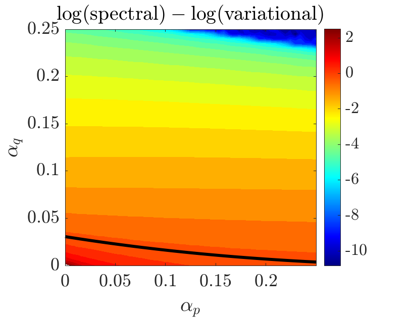
As expected, for large numbers of observations (small \(\alpha_p,\alpha_q\)), the variational method leads to better performance due to a reduced bias, but for smaller numbers of observations, its increasing variance makes the spectral method preferable.
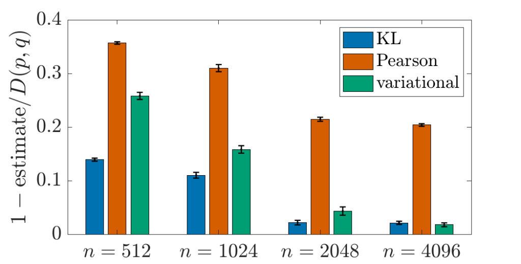
Simulations. We consider a simple situation with data in two dimensions (\(d=2\)) and a non-linear log-density which is learned using random features based on ReLUs, that is, \(\varphi(x)_i = (w_i^\top x + b_i)_+\) for \(i \in \{1,\dots,m\}\) for randomly chosen \((w_i,b_i) \in \mathbb{R}^{d+1}\), with an increasing number of observations \(n = n_p = n_q\). The problem of estimating KL divergence between generic distributions is a non-parametric problem with convergence rates that exhibit the curse of dimensionality, and unless \(n\) is very large, or special sparsity assumptions are made, we can only estimate accurately in small dimension (see below for higher dimension when feature learning is used).
We see that KL is better than using the Pearson divergence (which is the traditional way [22, 23, 24] to use least-squares for density estimation, but suffers from the improper geometry in particular in the way it deals with positivity of densities), and better than variational, except for a large number of observations, where variational and KL spectral are the same.
Mutual information and conditional estimation
Within information theory, the KL divergence is often used as a measure of independence between random variables, leading to the mutual information: given a product space \(\mathcal{X}_1 \times \mathcal{X}_2\) and a joint distribution \(p(x_1,x_2)\), we can consider \(q(x_1,x_2)\) as the distribution with independent components that have the same marginals as \(p\), which we write \(q(x_1,x_2) = p(x_1) p(x_2)\), following the usual graphical model convention. Then the optimal log-relative-density is $$ \log \frac{ p(x_1,x_2)}{p(x_2) p(x_1)} = \log \frac{ p(x_2|x_1)}{p(x_2)}.$$
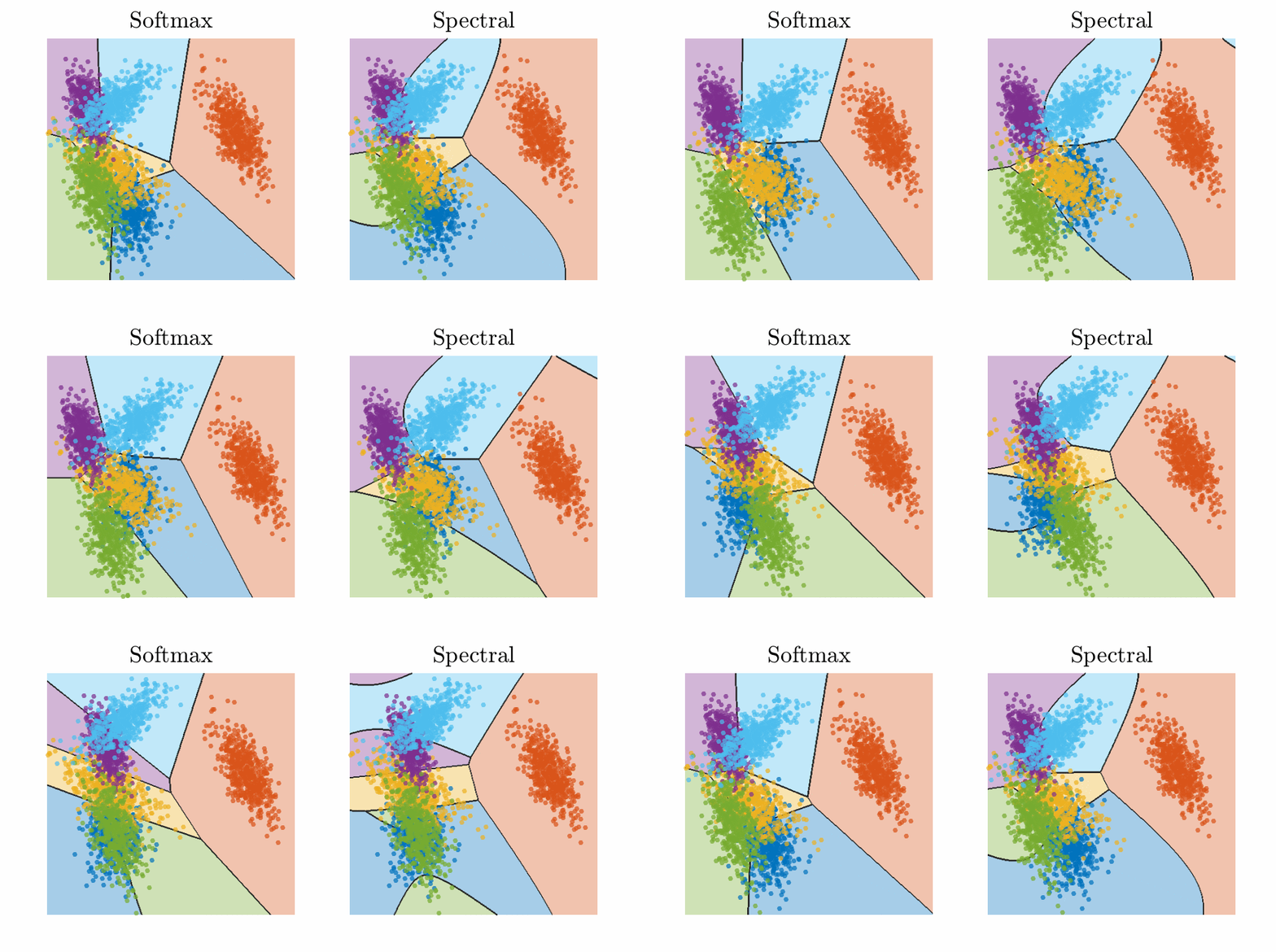
Hence, our framework for closed-form estimation allows us to perform conditional density estimation \(\log p(x_2|x_1)\) (with the additional need for \(\log p(x_2)\)). This can be done in general for any \(\mathcal{X}_2\), but when \(\mathcal{X}_2\) is finite, our closed-form estimation is exactly a way to perform softmax regression.
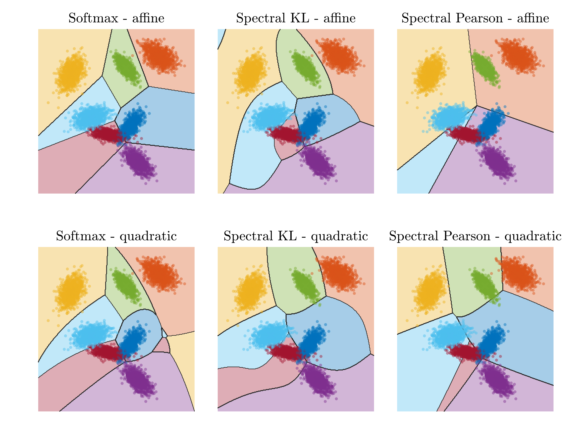
It is also interesting to consider adding quadratic features (because the log-density here is quadratic since the class-conditional covariance matrices are not equal), and also compare to the classical square loss (which corresponds to using Pearson divergence, that is, \(\nu\) is a Dirac at \(\rho=0\)). With more features, all methods tend to have more similar classification regions (if the set of features is big enough to model all real-valued functions, they are identical). Note that on the top right, we see the masking problem of least-squares where some classes totally disappear (this is solved by adding features in the bottom right plot, but indicates an unnatural cost function).
Computational complexity. To obtain estimates with machine precision for \(k\) classes with feature vectors in dimension \(d\), then softmax regression using Newton’s method would take \(O( nd^2 k^2 + d^3 k^3)\) per Newton iteration, while the closed-form estimator takes only \(O(d^2 n + kd^3)\) for one eigenvalue decomposition, which is a significant gain. When gradient-based algorithms are used with feature learning, both computation times can be reduced.
Feature learning
Linear models are great, but if one lesson has been learned since deep learning took over, it is that we need to learn features in a more end-to-end way, and large sets of predefined features are not enough for various reasons, in particular adaptivity to unknown (linear or non-linear) latent variables. In our variational framework where we have a lower bound on the KL divergence, this is simply maximizing \(F(p\|q, \varphi)\) in Eq. (7) with respect to \(\varphi\), and leveraging the fact that \(F(p\|q, \varphi)\) is convex in moments of \(\varphi\).
Indeed, as a convex function of the moments \(\mu_p-\mu_q,\Sigma_p,\Sigma_q\), it is lower-bounded by a constant plus $$ {\rm tr} \big( M \mathbb{E}_p [ \varphi \varphi^\top ] \big) + {\rm tr} \big( N \mathbb{E}_q [ \varphi \varphi^\top ] \big) + 2c^\top \big( \mathbb{E}_p [\varphi] – \mathbb{E}_q[\varphi]),$$ for matrices \(M,N\) and a vector \(c\) which can be computed from any given \(\bar\varphi\) (this is exactly what was needed to compute the potentials \(v\) and \(w\), and chosen so that the lower bound is tight for \(\varphi = \bar\varphi\) (see the section below the references). This allows for a minorization-maximization algorithm [15, 16] similar to the expectation-maximization (EM) algorithm [17]. The link with EM allows us to reuse many of the computational tricks developed there, such as online EM [18], to make the algorithm scalable to large networks to parameterize \(\varphi\) and large numbers of observations. More on this in a next post.
Conclusion
In this blog post, I introduced a new framework for relative density estimation that circumvents the exploding variance of means of exponentials. This was obtained by a continuum of stable least-squares problems, and made computationally feasible through a single generalized eigenvalue decomposition. Beyond tackling the exploding variance problem for models that need to be normalized, the unintended consequence for normalized models (where the sum/integral can be computed) was to obtain a closed-form estimator for softmax regression.
The recent paper [7] explores other consequences, in particular in terms of rates of estimation for the KL divergence, sometimes with minimax rates and partial adaptivity to linear latent variables. Overall, there is a long way to go, but I see this new framework as a potential replacement for the last layer of neural networks, where cross-entropy loss and log-sum-exp dominate. More on this in the next post.
Acknowledgements and tool usage disclosure. I would like to thank Frederik Kunstner and Nicolas Flammarion for helpful clarifying suggestions. Frontier LLM models were used to produce figures and correct typos.
References
[1] XuanLong Nguyen, Martin J. Wainwright, and Michael I. Jordan. Estimating divergence functionals and the likelihood ratio by convex risk minimization. IEEE Transactions on Information Theory, 56(11):5847–5861, 2010.
Playing with SDPs
We defined our new divergence in Eq. (7) as $$F(p\|q,\varphi) = \frac{1}{2} \int_0^1 ( \mu_p \, – \mu_q)^\top( \rho \Sigma_p + (1-\rho) \Sigma_q)^{-1} ( \mu_p\, – \mu_q) d\nu(\rho). $$ It is convex in \(\Sigma_p\), \(\Sigma_q\), and \(\mu_p – \mu_q\), and there is a nice duality theory here, showing that \(M,N,2c\) defined above are in fact derivatives with respect to the parameters above. The main result here, shown in [7], is: $$F(p\|q,\varphi) = \ \sup_{M,N,c} {\rm tr}(\Sigma_p M) + {\rm tr}(\Sigma_q N) + 2c^\top (\mu_p – \mu_q) \qquad \qquad \qquad \qquad$$ $$\qquad \qquad \qquad \qquad \mbox{ such that } \ \forall \lambda \geqslant 0, \left( \begin{array}{cc} \lambda M + N & (\lambda-1)c \\ (\lambda-1)c^\top & -f(\lambda) \end{array} \right) \preccurlyeq 0.$$ The semi-definite constraint above exactly implies that the potentials \(v(x)\) and \(w(x)\) are such that \(\forall x \in \mathcal{X}, \ w(x) + f^\ast(v(x)) \leqslant 0\), in exactly the same way as semi-definite programming can be used for optimization through sums-of-squares (see, e.g., [10]). Indeed, for any \(\lambda \geqslant 0\), we have $$\lambda v(x) + w(x) -f(\lambda) = { \varphi(x) \choose 1}^\top \left( \begin{array}{cc} \lambda M + N & (\lambda-1)c \\ (\lambda-1)c^\top & -f(\lambda) \end{array} \right) { \varphi(x) \choose 1} \leqslant 0,$$ which is equivalent to \(w(x) + f^\ast(v(x)) \leqslant 0\).
In earlier work [20], I had developed a similar framework for feature maps that were normalized so that \(\| \varphi(x)\|=1\), leading to the lower bound on \(D(p\|q)\) equal to $$\sup_{M,N} {\rm tr}(\Sigma_p M) + {\rm tr}(\Sigma_q N) \ \mbox{ such that } \ \forall \lambda \geqslant 0, \ \lambda M + N + f(\lambda) I \preccurlyeq 0, $$ which is then equal to an expression common in quantum information theory [21], that is, $$ {\rm tr} \big[ \Sigma_q f( \Sigma_q^{-1/2} \Sigma_p \Sigma_q^{-1/2})\big].$$ The key novelty is that we no longer need normalized features, which makes feature learning significantly easier.