James Routley

This is the fascinating story of how researchers used Bloom filters cleverly to make SQLite 10x faster for analytical queries. These are my five-minute notes on the paper SQLite: Past, Present, and Future (2022). I’ll also explain some database internals and how databases implement joins.

Background

SQLite is a B-tree on disk, row-based storage. It internally uses a VM called VDBE to execute queries. It is cross-platform, single-threaded, and runs almost everywhere.

SQLite is a general-purpose database, but it excels at OLTP workloads. However, researchers at Buffalo University in 2015 found that most queries are simple key-value lookups and complicated OLAP queries. So, researchers at the University of Wisconsin-Madison set out to make it faster for analytical queries since the trend is changing. To set a baseline, they used DuckDB. They used the industry standard OLAP benchmark - Star Schema Benchmark (SSB).

SSB contains a bunch of analytical queries called Star Queries, where you have one large fact table and multiple smaller dimension tables. e.g., fact table = customer orders, dimension tables = customer, merchant info, delivery partners, etc.

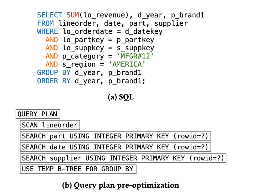
Here is a sample query with the query plan. Like a typical analytical query, this one contains joins between four tables.

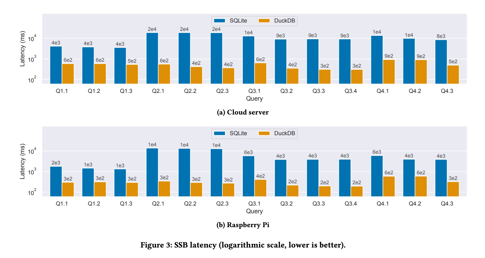
As expected, they found DuckDB to be 30-50x faster than SQLite. Note that they ran DuckDB in single-threaded mode.

Cause

Let’s figure out why SQLite was slow; then, we can determine how to make it faster. SQLite has a compile time option, VDBE_PROFILE, which measures the number of CPU cycles each instruction takes in VDBE. When they reran the benchmarks, they found two opcodes:

What do these opcodes do?

SeekRowID - given a rowId, probe the row in B-tree
Column - extract a column from a given record

Since the analytical queries mainly contain join operations, let’s understand how they are implemented.

Database Joins

Following are some of the ways databases implement joins:

Nested Loop Joins
Hash Joins
Sort-Merge Join

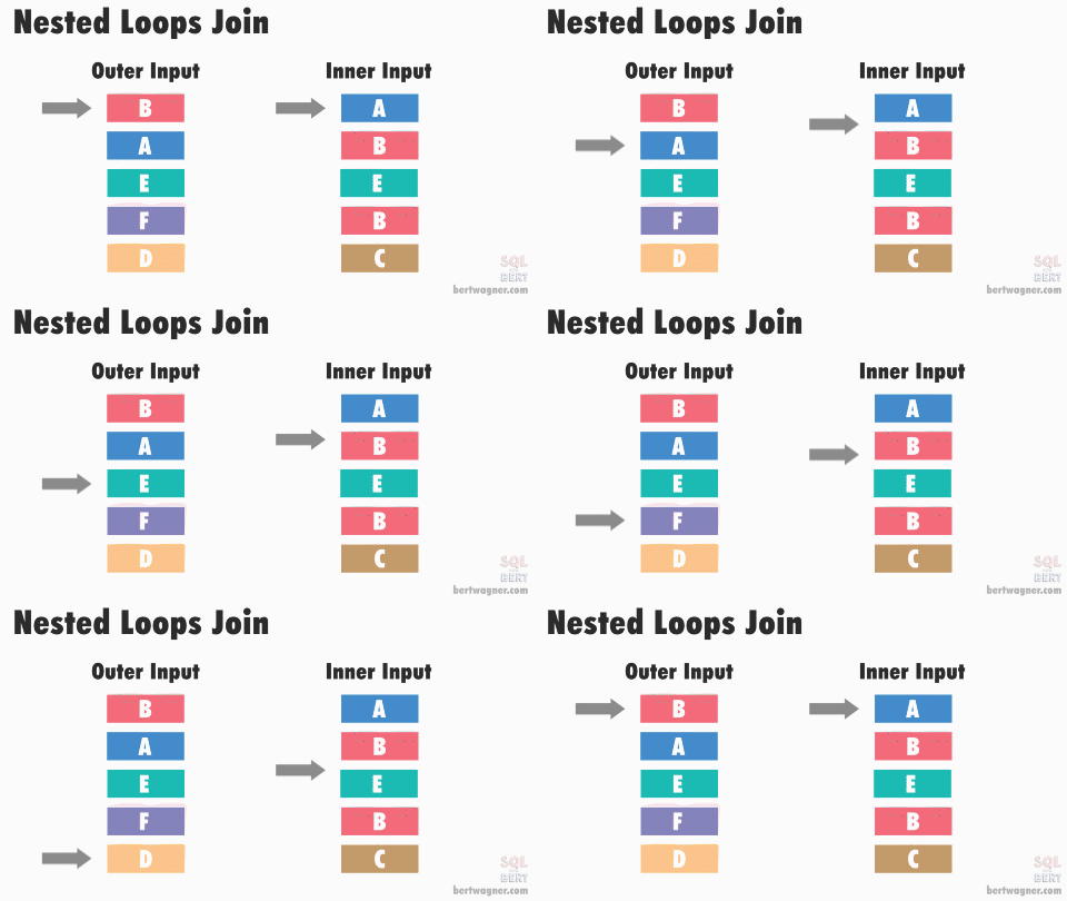
SQLite does Nested Loop join, which is the simplest of all three. Here is an animation (source) showing how Nested Loop join works:

Here is a sample Python-like pseudocode:

orders: {id, data} = [(1, obj...), (7, ...), (21, ...)] # fact table
customers: {order_id, data} = [(2, obj...), (7, ...), (14, ...)] # dimension table

selected = []
for order in orders:
    for customer in customers:
        # discards data when customer is 2 or 14
        if order.id == customer.order_id:
            selected.append(customer)

Assume you have two tables: orders and customers. The code here depicts joining both tables using the order_id column. The outer loop iterates over every item in the customers table, and for each item, it iterates over every item in the orders table.

For every id it matches, it appends to the result list. The loop operations are equivalent to probing in B-tree, which is very expensive.

Your goal is to reduce the B-tree probes. Now, stop for a minute and consider why this is not good. Can you come up with some ideas where you can make this better?

Join Order

Next, the order of tables in the join operation matters. Here is a simple illustration:

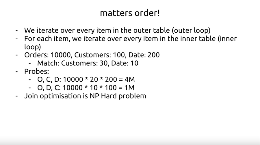
Consider there are three tables: Orders, Customers, Date. Our query matches 20 items in Customers and 10 items in Date. We probe the B-tree whenever a row matches.

O, C, D: 10000 * 20 * 200 = 4M
O, D, C: 10000 * 10 * 100 = 1M

Just by flipping the order, it reduced to 1M operations! But it is incredibly difficult to come up with an optimized query plan. It is an NP-Hard problem.

Optimization

How do we optimize the join? The other two join algorithms are better than Nested Loop join. However, authors argue that Hash Join takes significant memory, and SQLite mostly runs in memory-constrained environments. Second, adding one more join algorithm would complicate the query planner.

orders = [(1, obj...), (7, ...), (21, ...)]
customers = [(2, obj...), (7, ...), (14, ...)]

selected = []
cache = {2: True, 7: True, 14: True}
for order in orders:
    if order.id in cache:
        # we only check customers at cache hit
        for customer in customers:
            if order.id == customer.order_id:
                selected.append(customer)

Here is one way: before you run both loops, you first build the customer data cache. Then, in the inner loop, first, you check this cache. Only if there is a match do you iterate over the loop.

That’s what the researchers did! They used a Bloom filter, which is very space efficient and fits in a CPU cache line. It was also easy to implement.

They added two opcodes: Filter and FilterAdd. At the start of the join operation, we go over all the rows of dimension tables and set the bits in the Bloom filter which match the query predicate. The opcode is FilterAdd.

During the join operation, we first check if the row exists in the Bloom filter at each stage. If it does, then we do the B-tree probe. This is the Filter opcode.

Results

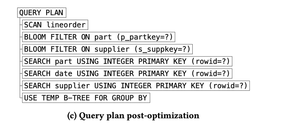
This is the optimized query plan.

This is the CPU cycle analysis post-optimization. You can see that the large blue bars are almost gone!

The result? SQLite became 7x-10x faster!

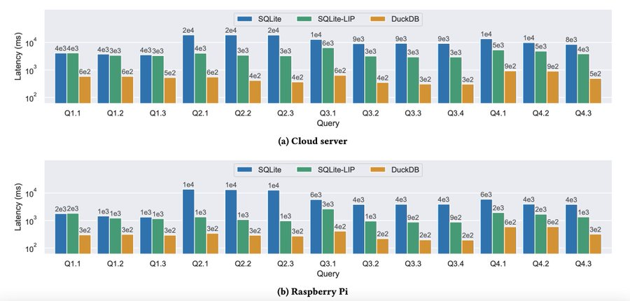
The results of this research have been applied to SQLite already and were released in v3.38.0.

tl;dr: Bloom filters were great because: minimal memory overhead, goes well with SQLite’s simple implementation, and worked within existing query engine.

1. I presented this paper at a local Papers We Love group. This blog post is a summary of the talk