Nano-vLLM: How a vLLM-style inference engine works

Architecture, Scheduling, and the Path from Prompt to Token

When deploying large language models in production, the inference engine becomes a critical piece of infrastructure. Every LLM API you use — OpenAI, Claude, DeepSeek — is sitting on top of an inference engine like this. While most developers interact with LLMs through high-level APIs, understanding what happens beneath the surface—how prompts are processed, how requests are batched, and how GPU resources are managed—can significantly impact system design decisions.

This two-part series explores these internals through Nano-vLLM, a minimal (~1,200 lines of Python) yet production-grade implementation that distills the core ideas behind vLLM, one of the most widely adopted open-source inference engines.

Nano-vLLM was created by a contributor to DeepSeek, whose name appears on the technical reports of models like DeepSeek-V3 and R1. Despite its minimal codebase, it implements the essential features that make vLLM production-ready: prefix caching, tensor parallelism, CUDA graph compilation, and torch compilation optimizations. Benchmarks show it achieving throughput comparable to—or even slightly exceeding—the full vLLM implementation. This makes it an ideal lens for understanding inference engine design without getting lost in the complexity of supporting dozens of model architectures and hardware backends.

In Part 1, we focus on the engineering architecture: how the system is organized, how requests flow through the pipeline, and how scheduling decisions are made. We will treat the actual model computation as a black box for now—Part 2 will open that box to explore attention mechanisms, KV cache internals, and tensor parallelism at the computation level.

The Main Flow: From Prompt to Output

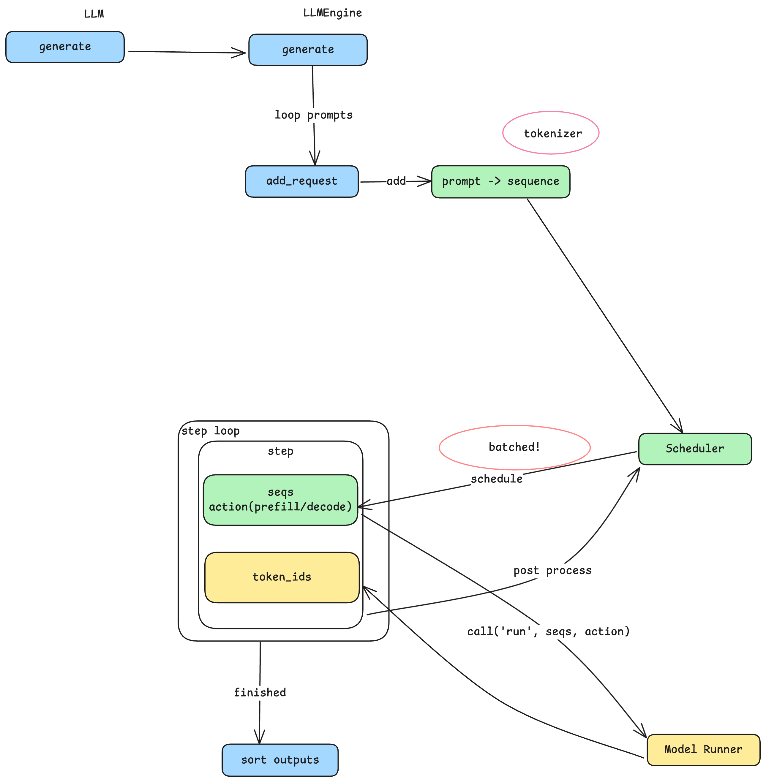
The entry point to Nano-vLLM is straightforward: an LLM class with a generate method. You pass in an array of prompts and sampling parameters, and get back the generated text. But behind this simple interface lies a carefully designed pipeline that transforms text into tokens, schedules computation efficiently, and manages GPU resources.

From Prompts to Sequences

When generate is called, each prompt string goes through a tokenizer—a model-specific component that splits natural language into tokens, the fundamental units that LLMs process. Different model families (Qwen, LLaMA, DeepSeek) use different tokenizers, which is why a prompt of the same length may produce different token counts across models. The tokenizer converts each prompt into a sequence: an internal data structure representing a variable-length array of token IDs. This sequence becomes the core unit of work flowing through the rest of the system.

The Producer-Consumer Pattern

Here’s where the architecture gets interesting. Rather than processing each sequence immediately, the system adopts a producer-consumer pattern with the Scheduler at its center. The add_request method acts as the producer: it converts prompts to sequences and places them into the Scheduler’s queue. Meanwhile, a separate step loop acts as the consumer, pulling batches of sequences from the Scheduler for processing. This decoupling is key—it allows the system to accumulate multiple sequences and process them together, which is where the performance gains come from.

Batching and the Throughput-Latency Trade-off

Why does batching matter? GPU computation has significant fixed overhead—initializing CUDA kernels, transferring data between CPU and GPU memory, and synchronizing results. If you process one sequence at a time, you pay this overhead for every single request. By batching multiple sequences together, you amortize this overhead across many requests, dramatically improving overall throughput.

However, batching comes with a trade-off. When three prompts are batched together, each must wait for the others to complete before any results are returned. The total time for the batch is determined by the slowest sequence. This means: larger batches yield higher throughput but potentially higher latency for individual requests; smaller batches yield lower latency but reduced throughput. This is a fundamental tension in inference engine design, and the batch size parameters you configure directly control this trade-off.

Prefill vs. Decode: Two Phases of Generation

Before diving into the Scheduler, we need to understand a crucial distinction. LLM inference happens in two phases:

• Prefill: Processing the input prompt. All input tokens are processed together to build up the model’s internal state. During this phase, the user sees nothing.
• Decode: Generating output tokens. The model produces one token at a time, each depending on all previous tokens. This is when you see text streaming out.

For a single sequence, there is exactly one prefill phase followed by many decode steps. The Scheduler needs to distinguish between these phases because they have very different computational characteristics—prefill processes many tokens at once, while decode processes just one token per step.

Inside the Scheduler

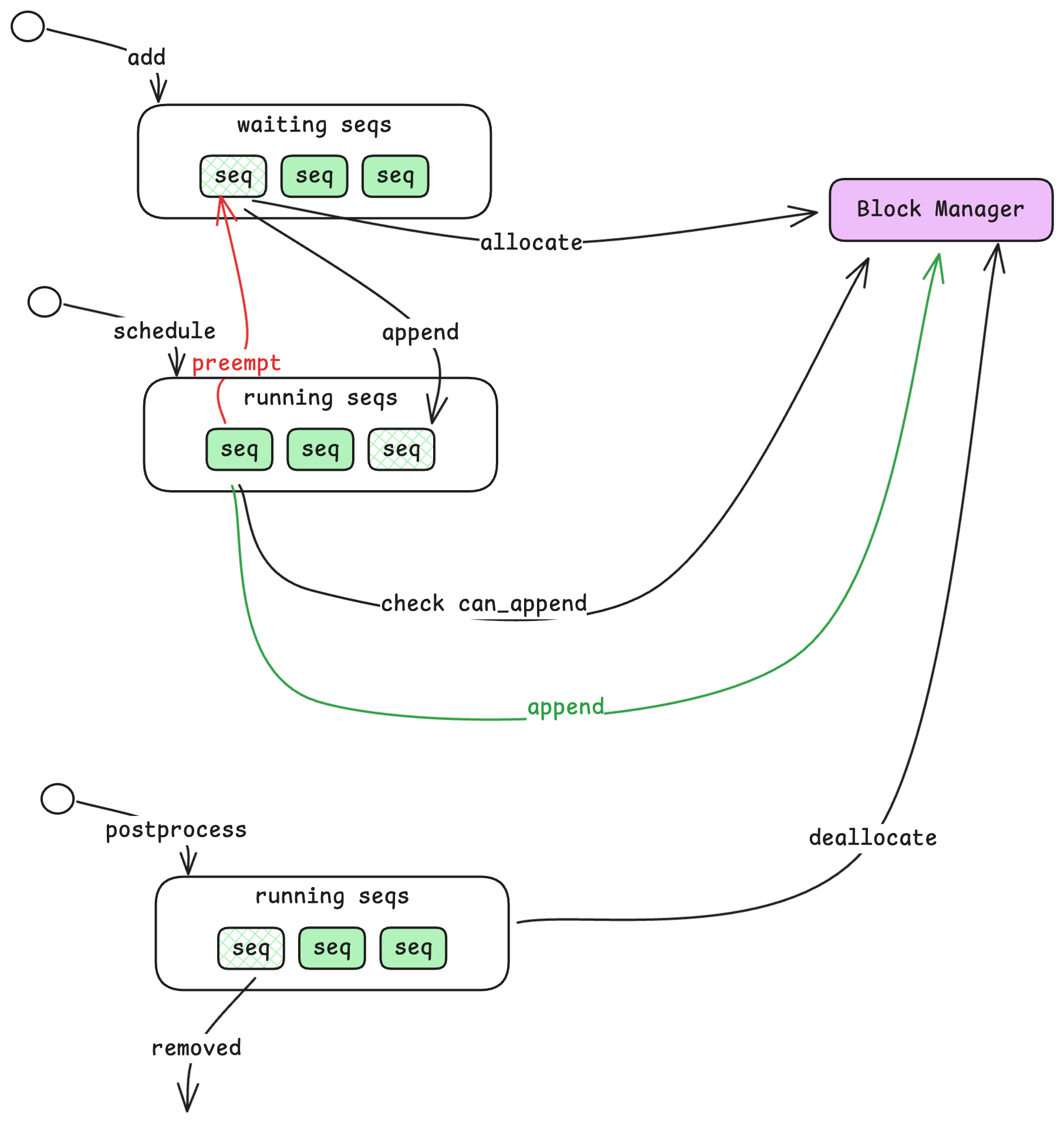
The Scheduler is responsible for deciding which sequences to process and in what order. It maintains two queues:

Waiting and Running Queues

• Waiting Queue: Sequences that have been submitted but not yet started. New sequences from add_request always enter here first.
• Running Queue: Sequences that are actively being processed—either in prefill or decode phase.

When a sequence enters the Waiting queue, the Scheduler checks with another component called the Block Manager to allocate resources for it. Once allocated, the sequence moves to the Running queue. The Scheduler then selects sequences from the Running queue for the next computation step, grouping them into a batch along with an action indicator (prefill or decode).

Handling Resource Exhaustion

What happens when GPU memory fills up? The KV cache (which stores intermediate computation results) has limited capacity. If a sequence in the Running queue cannot continue because there’s no room to store its next token’s cache, the Scheduler preempts it—moving it back to the front of the Waiting queue. This ensures the sequence will resume as soon as resources free up, while allowing other sequences to make progress.

When a sequence completes (reaches an end-of-sequence token or maximum length), the Scheduler removes it from the Running queue and deallocates its resources, freeing space for waiting sequences.

The Block Manager: KV Cache Control Plane

The Block Manager is where vLLM’s memory management innovation lives. To understand it, we first need to introduce a new resource unit: the block.

From Sequences to Blocks

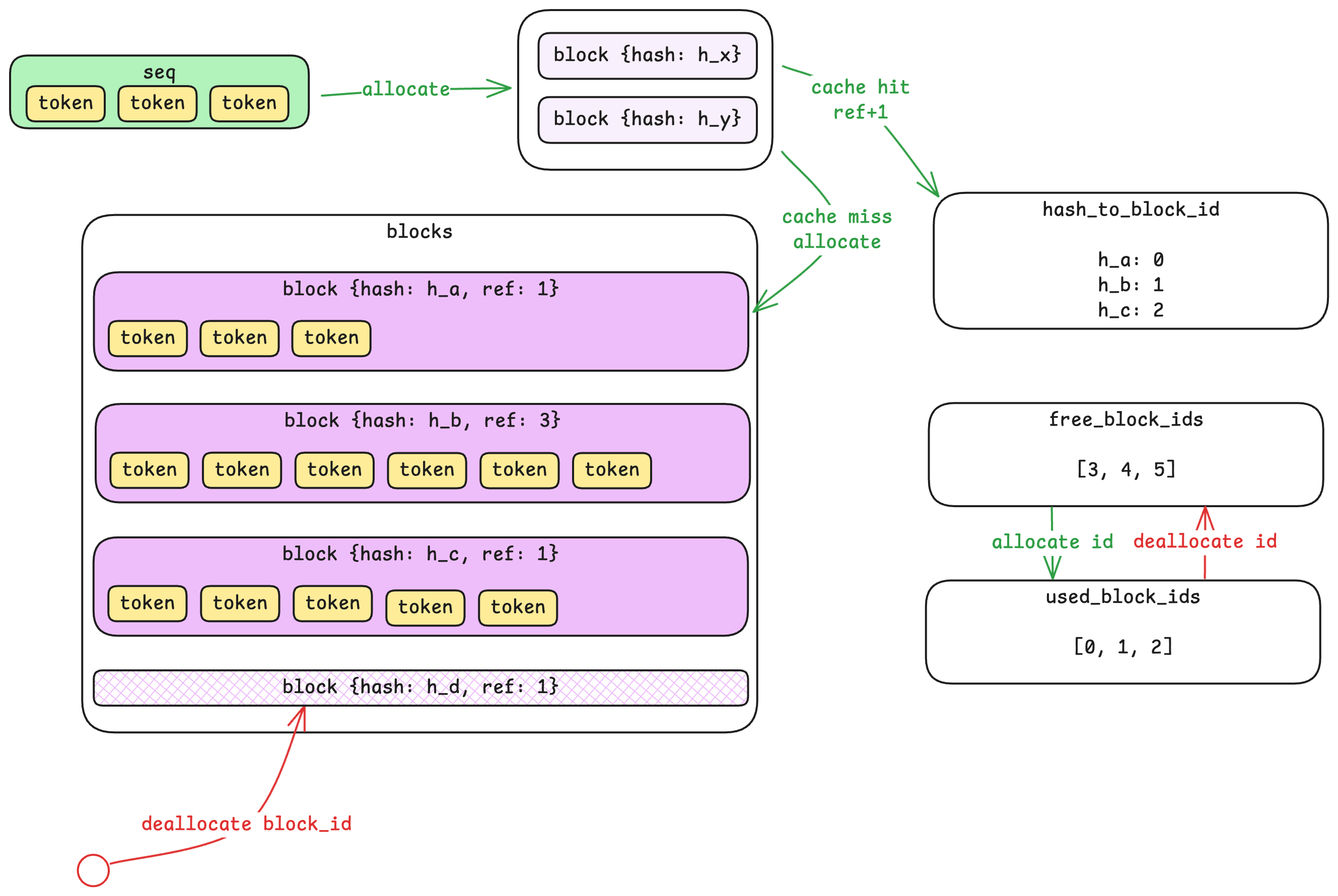
A sequence is a variable-length array of tokens—it can be 10 tokens or 10,000. But variable-length allocations are inefficient for GPU memory management. The Block Manager solves this by dividing sequences into fixed-size blocks (default: 256 tokens each).

A 700-token sequence would occupy three blocks: two full blocks (256 tokens each) and one partial block (188 tokens, with 68 slots unused). Importantly, tokens from different sequences never share a block—but a long sequence will span multiple blocks.

Prefix Caching via Hashing

Here’s where it gets clever. Each block’s content is hashed, and the Block Manager maintains a hash-to-block-id mapping. When a new sequence arrives, the system computes hashes for its blocks and checks if any already exist in the cache.

If a block with the same hash exists, the system reuses it by incrementing a reference count—no redundant computation or storage needed. This is particularly powerful for scenarios where many requests share common prefixes (like system prompts in chat applications). The prefix only needs to be computed once; subsequent requests can reuse the cached results.

Control Plane vs. Data Plane

A subtle but important point: the Block Manager lives in CPU memory and only tracks metadata—which blocks are allocated, their reference counts, and hash mappings. The actual KV cache data lives on the GPU. The Block Manager is the control plane; the GPU memory is the data plane. This separation allows fast allocation decisions without touching GPU memory until actual computation happens.

When blocks are deallocated, the Block Manager marks them as free immediately, but the GPU memory isn’t zeroed—it’s simply overwritten when the block is reused. This avoids unnecessary memory operations.

The Model Runner: Execution and Parallelism

The Model Runner is responsible for actually executing the model on GPU(s). When the step loop retrieves a batch of sequences from the Scheduler, it passes them to the Model Runner along with the action (prefill or decode).

Tensor Parallel Communication

When a model is too large for a single GPU, Nano-vLLM supports tensor parallelism (TP)—splitting the model across multiple GPUs. With TP=8, for example, eight GPUs work together to run a single model.

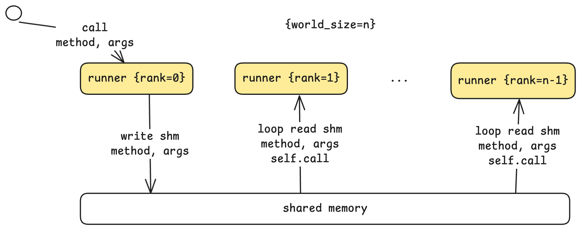
The communication architecture uses a leader-worker pattern:

• Rank 0 (Leader): Receives commands from the step loop, executes its portion, and coordinates with workers.
• Ranks 1 to N-1 (Workers): Continuously poll a shared memory buffer for commands from the leader.

When the leader receives a run command, it writes the method name and arguments to shared memory. Workers detect this, read the parameters, and execute the same operation on their respective GPUs. Each worker knows its rank, so it can compute its designated portion of the work. This shared-memory approach is efficient for single-machine multi-GPU setups, avoiding network overhead.

Preparing for Computation

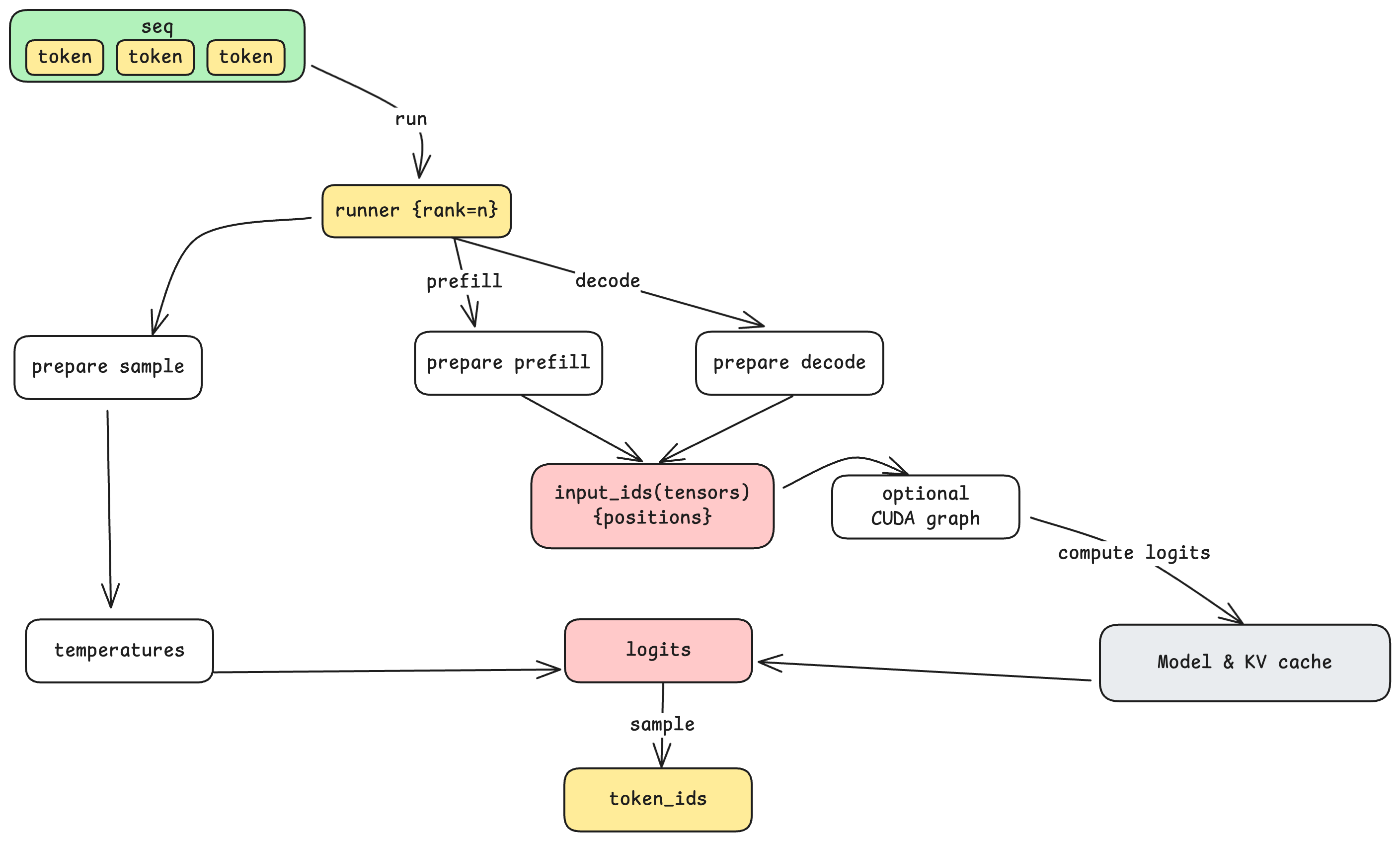
Before invoking the model, the Model Runner prepares the input based on the action:

• Prepare Prefill: Batches multiple sequences with variable lengths, computing cumulative sequence lengths for efficient attention computation.
• Prepare Decode: Batches single tokens (one per sequence) with their positions and slot mappings for KV cache access.

This preparation also involves converting CPU-side token data into GPU tensors—the point where data crosses from CPU memory to GPU memory.

CUDA Graphs: Reducing Kernel Launch Overhead

For decode steps (which process just one token per sequence), kernel launch overhead can become significant relative to actual computation. CUDA Graphs address this by recording a sequence of GPU operations once, then replaying them with different inputs. Nano-vLLM pre-captures CUDA graphs for common batch sizes (1, 2, 4, 8, 16, up to 512), allowing decode steps to execute with minimal launch overhead.

Sampling: From Logits to Tokens

The model doesn’t output a single token—it outputs logits, a probability distribution over the entire vocabulary. The final step is sampling: selecting one token from this distribution.

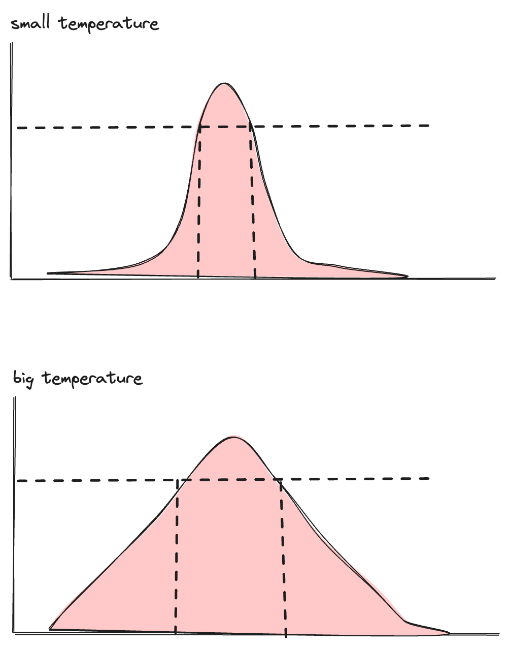
The temperature parameter controls this selection. Mathematically, it adjusts the shape of the probability distribution:

• Low temperature (approaching 0): The distribution becomes sharply peaked. The highest-probability token is almost always selected, making outputs more deterministic and focused.
• High temperature: The distribution flattens. Lower-probability tokens have a better chance of being selected, making outputs more diverse and creative.

This is where the “randomness” in LLM outputs comes from—and why the same prompt can produce different responses. The sampling step selects from a valid range of candidates, introducing controlled variability.

What’s Next

In Part 2, we’ll open the black box of model. We’ll explore:

• How the model transforms tokens into hidden states and back
• The attention mechanism and why multi-head attention matters
• How KV cache is physically laid out on GPU memory
• Dense vs. MoE (Mixture of Experts) architectures
• How tensor parallelism works at the computation level

Understanding these internals will complete the picture—from prompt string to generated text, with nothing left hidden.