Last week we released version 0.2 of pgrust. This release was all about performance. It’s 10x faster than the previous version of pgrust. On OLTP benchmarks, pgrust is 30% faster than Postgres, and on Clickbench, Clickhouse’s benchmark for analytical databases, pgrust is 300x faster than Postgres. It’s even ahead of Clickhouse!
The query engine is one of the biggest changes we made to achieve much better performance. On its own, the query engine drove ~10x of the 300x. We’ll start with a miniature version of the Postgres query engine and we’ll one by one add the same optimizations we made to make the pgrust query engine so fast.
To give some background on why there’s so much room for improvement vs Postgres, Postgres was created in a different era. The original Postgres project dates back to the 80s. It was built at a time when the main bottleneck to database performance was disk I/O. Three trends have made that no longer the case:
- Many datasets now fit in RAM, eliminating most disk I/O
- For datasets that don’t fit in RAM, the workloads differ. Data analytics scans data in bulk. The bottleneck is often no longer your disk throughput and is often either your CPU throughput or memory throughput
- Disks have gotten much faster in recent years. NVMe is hundreds of times faster than a hard drive.
All three trends have made CPU and memory speeds more important than they were historically. Many of the optimizations we’ve made target this. The query engine is the main user of CPU in a database. We optimized the pgrust query engine to use less CPU and less memory bandwidth than Postgres when processing the same queries.
To give you a sense of just how slow the Postgres query engine is, let’s take a simple query that sums the first 500 million numbers:
CREATE TABLE my_table AS select col::float8 from generate_series(1.0, 500000000.0) g(col);
SELECT SUM(col) FROM my_table;
When I run this in Postgres, it takes ~20 seconds. This was done on a c8g.4xl with parallel queries disabled.
For comparison, when I time the equivalent in Rust:
let table: Vec<f64> = (1..=500_000_000usize).map(|i| i as f64).collect();

let mut sum = 0.0;
for &value in &table {
    sum += value;
}
The query takes 358ms. That’s around 55x faster, and believe it or not, we can do even faster than 358ms. Now this example isn’t an apples-to-apples comparison. There’s a lot more going on under the hood in Postgres. At the same time, optimizing a database is all about removing as much of this overhead as possible. (If you’re curious two of the biggest causes of overhead from Postgres are 1. locking and 2. parsing the Postgres storage format and extracting the tuples relevant to the query).
To narrow our focus to just the impact of the query engine, let’s build a miniature version of the Postgres query engine. First, a brief explanation of what a query engine is. When processing your SQL query, Postgres first converts your query into an internal representation called a “Query Plan,” which describes *how* Postgres will execute the query. In the example above, Postgres will produce a query plan that may look something like the following:
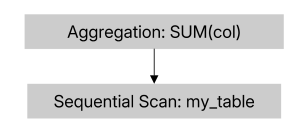
This effectively says “get rows from my_table and sum the values in those rows”. This query plan is pretty simple given the nature of the query, but they can get much more complicated when you start working with joins/sorts/subqueries etc. In total Postgres has over 40 different types of plan nodes.
After generating the query plan, Postgres passes it to the query engine. The Postgres query engine is the part of Postgres that takes the query plan and actually retrieves the rows and performs the aggregation. Postgres uses a style of executor known as the “Volcano model.” To get a sense of how it works, here’s a miniature implementation of the Postgres query engine:
use std::hint::black_box;

trait Node {
    fn next(&mut self) -> Option<f64>;
}

struct SeqScan<'a> {
    table: &'a [f64],
    pos: usize,
}

impl Node for SeqScan<'_> {
    fn next(&mut self) -> Option<f64> {
        if self.pos >= self.table.len() {
            return None; // end of table
        }
        let value = self.table[self.pos];
        self.pos += 1;
        Some(value)
    }
}

struct SumAggregate<'a> {
    child: Box<dyn Node + 'a>,
    total: f64,
    done: bool,
}

impl Node for SumAggregate<'_> {
    fn next(&mut self) -> Option<f64> {
        if self.done {
            return None;
        }
        while let Some(value) = self.child.next() {
            self.total += value;
        }
        self.done = true;
        Some(self.total)
    }
}

let table: Vec<f64> = (1..=500_000_000usize).map(|i| i as f64).collect();

let mut plan = SumAggregate {
    child: black_box(Box::new(SeqScan { table: &table, pos: 0 })),
    total: 0.0,
    done: false,
};

let sum = plan.next().unwrap();
(The black_box is needed to prevent compiler optimizations from thwarting our benchmark)
The key feature of the Volcano model is the `next()` method, which is supported by all nodes in the query plan. The job of `next()` is to return a single row. `next()` in a sequential scan returns the next row in the sequential scan. `next()` on an aggregation will compute the entire aggregation and then return the single row result. Executing a query plan is just a matter of calling `next()` on the root plan node until it no longer returns any rows. The advantage of the Volcano model is that it’s very simple. You implement a single method for each of your plan nodes, and that’s it. While simplified, the above code is very close to what Postgres does internally.
While the Volcano model makes things simple, it also adds a lot of overhead. When I run this example, it takes 1.3s. That’s much faster than the Postgres version because we’re removing a lot of the non-query engine pieces, but it’s still slower than the raw for loop because of the Volcano model’s overhead.
The biggest performance hit in the code above is that `next()` processes only one row at a time. There’s no batching. The `SeqScan.next()` function is called once per row. That adds significant overhead, especially because many CPU optimizations, such as pipelining, don’t work well when you are calling a function that isn’t known until runtime. The first optimization we can implement is batching:
const BATCH: usize = 1024;

trait BatchNode {
    fn next_batch(&mut self, out: &mut [f64; BATCH]) -> usize;
}

struct BatchSeqScan<'a> {
    table: &'a [f64],
    pos: usize,
}

impl BatchNode for BatchSeqScan<'_> {
    fn next_batch(&mut self, out: &mut [f64; BATCH]) -> usize {
        let n = (self.table.len() - self.pos).min(BATCH);
        out[..n].copy_from_slice(&self.table[self.pos..self.pos + n]);
        self.pos += n;
        n
    }
}

struct BatchSumAggregate<'a> {
    child: Box<dyn BatchNode + 'a>,
    total: f64,
}

impl BatchSumAggregate<'_> {
    fn run(&mut self) -> f64 {
        let mut buf = [0.0f64; BATCH];
        loop {
            let n = self.child.next_batch(&mut buf);
            if n == 0 {
                break;
            }
            for &value in &buf[..n] {
                self.total += value;
            }
        }
        self.total
    }
}

let mut plan = BatchSumAggregate {
    child: black_box(Box::new(BatchSeqScan { table: &table, pos: 0 })),
    total: 0.0,
};
let sum = plan.run();
Batching on its own eliminates most of the overhead. It brings the time to run the query from 1.3 seconds down to around 480ms. Still slower than the for loop, but much closer. One very important detail is that the batch buffer is allocated on the stack. This means the aggregation node doesn’t need to allocate any memory while it’s running. Allocating memory tends to be one of the slower operations. Therefore, when writing ultra-fast code, you’ll want to minimize the number of memory allocations you make.
Now, if you profile the batched version, the hotspot is now `copy_from_slice`. Even though we are now batching, we still need to copy the items into the buffer. This overhead can be eliminated with what’s known as “operator fusion”. If there are common operations that we know will be performed together, we can create a single node that replaces two nodes. In our case, we can create a single `SumAggregateSequentialScan` node that combines the logic of both the sequential scan and the sum:
struct SumAggregateSequentialScan<'a> {
impl Node for SumAggregateSequentialScan<'_> {
This gives us the same performance as the straight for loop because it is literally the same code as the for loop. Now this may seem like cheating, and it definitely is because we’re hardcoding in an optimization for a specific query we know in advance. With operator fusion, it makes sense to hardcode a couple of the most common cases, but you’ll still pretty quickly hit cases you didn’t prepare for ahead of time.
This can be solved with JIT compilation. With JIT compilation, you can generate the ideal code you wish you had and “cheat” in every query. JIT compilation lets you generate the perfect code for your query, no matter what the query is and always do operator fusion. Unfortunately, this post is long enough as is, so I’ll have to talk about how pgrust leverages JIT compilation another time.
For one final optimization, we can look to SIMD. SIMD refers to a set of CPU operations that can perform one operation across multiple pieces of data simultaneously. Using SIMD to perform an operation against multiple rows simultaneously is usually much faster than performing the operation on one row at a time. If we change our code to use SIMD:
#[cfg(target_arch = "aarch64")]
struct SumAggregateSequentialScanSimd<'a> {
    table: &'a [f64],
    done: bool,
}

#[cfg(target_arch = "aarch64")]
impl Node for SumAggregateSequentialScanSimd<'_> {
    fn next(&mut self) -> Option<f64> {
        if self.done {
            return None;
        }
        self.done = true;
        use std::arch::aarch64::*;
        let mut acc = unsafe { [vdupq_n_f64(0.0); 4] };
        let (chunks, rest) = self.table.as_chunks::<8>();
        for chunk in chunks {
            for lane in 0..4 {
                unsafe {
                    let v = vld1q_f64(chunk.as_ptr().add(2 * lane));
                    acc[lane] = vaddq_f64(acc[lane], v);
                }
            }
        }
        let mut tail = 0.0;
        for &value in rest {
            tail += value;
        }
        Some(unsafe {
            let s01 = vaddq_f64(acc[0], acc[1]);
            let s23 = vaddq_f64(acc[2], acc[3]);
            vaddvq_f64(vaddq_f64(s01, s23)) + tail
        })
    }
}
Our code now takes 135ms which is now almost 3x faster than the for loop and 10x faster than our original Volcano code. While it is common for compilers to replace for loops with SIMD equivalents, I chose this example so that wouldn’t happen. Compilers will usually avoid introducing SIMD when operating on floats, because they will produce a slightly different result. This is because floating point arithmetic is not associative, so changing the order in which you do a sum can produce a slightly different result.
—
All in all, with three simple optimizations, we were able to make our query 10x faster. Here’s where things ended up:
| implementation | time | speedup |
|---|---|---|
| Postgres | ~20 s | — |
| Volcano model | 1.3 s | 1× |
| + batching | 480 ms | 2.7× |
| + operator fusion | 358 ms | 3.6× |
| + SIMD | 135 ms | 9.6× |
These types of optimizations, and many more, enable pgrust to perform hundreds of times faster than Postgres for analytical queries.
Benchmark setup: AWS c8g.4xlarge (Graviton4, 16 vCPU), PostgreSQL 18.4 with `max_parallel_workers_per_gather = 0`, data warm in shared buffers, median of 5 runs. Rust built with `cargo build –release`, 4 runs per implementation, all measured in one process on one machine.
Thanks for reading, and if you want to support the project, the best way to support pgrust is to give us a star on GitHub. If you want to follow along:
1. GitHub