I’ve been reading about renormalization lately. Not the physics kind, though. In 2024, Karl Friston and colleagues published a paper applying the renormalization group, one of the more celebrated ideas in theoretical physics, to generative image models. They called the result Renormalizing Generative Models, or RGMs. The paper is dense, but the core idea grabbed me, and I wanted to see if I could build a simplified version from scratch to understand it better, since that’s how I learn.
This post is the result. I don’t have a physics background, and my understanding of the renormalization group is shallow at best. What I’m presenting here is a “lite” version that captures what I think is the essential shape of the idea. I might be wrong about some of the finer points1.
This might sound like a lot, but if you have a rough sense of how a transformer tokenizes its input, that’s more than enough to follow along.
The complete code is on GitHub.
Why RGMs?
I believe RGMs are compelling because they offer a way to move from coarse to fine-grained descriptions and back again, operating at multiple levels, and it uses the same inference structure at every level. That’s cool because it means that abstraction and long-horizon behavior fall out naturally from the model being renormalizable, so the model can perceive, compress, and plan using one consistent story instead of a pile of task-specific hacks. Having the same formalism do classification, compression, generation, and planning is just an insanely cool thing.
Zooming out
So what is the idea? Start with something familiar: tokenization. If you’ve seen a Vision Transformer, you know the move: chop an image into patches, embed them, feed them into the model. RGMs start from the same place but go somewhere else entirely. Instead of learning relationships between tokens end-to-end through attention, you learn a hierarchy of tokens, where each level is a coarser summary of the level below it.
Think about how you recognize a handwritten digit. You don’t compare pixel-by-pixel against a template. You see strokes and curves first, then how those strokes are arranged relative to each other, and then you match that arrangement against your mental model of what a 3 or a 7 look like. There are at least two scales there: local shape, and global arrangement. That’s the hierarchy an RGM tries to make explicit.
Concretely: you take an image, tile it into small patches, and assign each patch to the nearest entry in a learned codebook. These are your tokens. Then you take neighboring groups of tokens and assign each group to a coarser codebook. These are your “supertokens”. Classification becomes a question of which digit class best explains the supertoken pattern you observe.
The renormalization part is the coarsening step: you’re replacing fine-grained detail with a coarser summary while preserving the spatial structure. In physics, the renormalization group is about doing this repeatedly and studying what survives, the idea being that the structure that persists across scales is the structure that matters. In my implementation we only do it once (two levels total), which is enough for MNIST but probably wouldn’t get you very far on harder problems.
The whole thing is a Bayesian hierarchy with closed-form updates. No backprop, no gradient descent. You fit it by counting. If that sounds too simple—it probably is, for anything beyond small grayscale digits. But it’s fast, interpretable, and the accuracy on MNIST is decent enough to suggest the idea isn’t totally theoretical.
Patches and tokens
We’re working with MNIST, so our input is a 28x28 grayscale image of a handwritten digit. The first thing we do is downsample it to 16x16. Purely pragmatic. Sixteen divides cleanly by four, which gives us a nice 4x4 grid of 4x4 patches. Smaller images also mean everything runs faster, and for MNIST the loss of resolution doesn’t hurt much2.
Once we have a 16x16 image, we tile it into non-overlapping 4x4 patches and flatten each one into a 16-dimensional vector:
def extract_patches(img, patch=4):
    H, W = img.shape; ph = pw = patch
    rows, cols = H // ph, W // pw
    patches = []
    for i in range(rows):
        for j in range(cols):
            block = img[i*ph:(i+1)*ph, j*pw:(j+1)*pw]
            patches.append(block.reshape(-1))
    return np.stack(patches, axis=0)  # [rows*cols, ph*pw]
Fig. 1: Patch extraction.
Each patch is a small piece of the digit—a stroke fragment, a curve, a blank region. Now we need a vocabulary: a set of prototypical patches—a codebook—so we can describe any patch by pointing to its nearest prototype. This is just K-means. We collect patches from the training set, standardize each one (zero mean, unit variance), and cluster them:
def standardize(p):
    mu = p.mean(1, keepdims=True); sd = p.std(1, keepdims=True) + 1e-6
    return (p - mu) / sd, mu.squeeze(1), sd.squeeze(1)

def fit_codebook_tokens(images_ds, K=256, bg_threshold=0.10, seed=42):
    fg = []
    for x in images_ds:
        p = extract_patches(x, patch=4)
        m = p.mean(1)
        p = p[m > bg_threshold]           # keep foreground patches only
        if len(p): fg.append(standardize(p)[0])
    X = np.vstack(fg)
    return kmeans(X, K, iters=25, seed=seed)
Fig. 2: Learning the token codebook.
We standardize each patch individually before clustering, which lets the codebook focus on shape rather than absolute brightness, since a dark stroke and a bright stroke with the same contour will map to the same centroid. And we filter out background patches so the codebook isn’t wasted on blank tiles. Most of an MNIST image is black; we don’t need 50 different codebook entries for “nothing”.
With K=256 we get a vocabulary of prototypical stroke
fragments. To tokenize an image, we extract its patches, standardize
them, and assign each one to its nearest centroid:
def tokens_grid(img_ds, codebook, patch=4):
    H, W = img_ds.shape
    rows, cols = H // patch, W // patch
    p = extract_patches(img_ds, patch=patch)
    pn, _, _ = standardize(p)
    z = ((pn[:, None, :] - codebook[None, :, :])**2).sum(2).argmin(1)
    return z.reshape(rows, cols)
Fig. 3: Tokenization via nearest centroid.
The result is a 4x4 grid of integers, each in the range
[0, 255]. We’ve gone from 256 floating-point pixel values
to 16 integers, a lossy compression that, ideally, keeps the structure
that matters for classification.
So far, this is a standard bag-of-visual-words setup. Nothing renormalization-specific yet.
The second scale
We now have a 4x4 grid of tokens. The renormalization move is to coarsen this grid: take non-overlapping 2x2 blocks of tokens and replace each block with a single “supertoken”. This is the block-spin analogy from physics: you group neighboring fine-grained variables and summarize them at a coarser scale.
To do this, we need a second codebook. For each 2x2 block of tokens, we look up the four token centroids and concatenate them into a 64-dimensional vector made up of 4 patches by 16 dimensions each. Then we standardize and do the same thing as before: collect from the training set, run K-means, get prototypes.
def block_features(z_grid, codebook):
    rows, cols = z_grid.shape
    feats = []
    for i in range(0, rows, 2):
        for j in range(0, cols, 2):
            ids4 = z_grid[i:i+2, j:j+2].ravel() # <- 4 token ids
            vec  = codebook[ids4].reshape(-1)   # <- concat centroids: 64 dims
            mu, sd = vec.mean(), vec.std() + 1e-6
            feats.append((vec - mu) / sd)
    return np.stack(feats, axis=0)
Fig. 4: Building supertoken features from 2x2 token blocks.
With K2=64, we get 64 supertoken prototypes. A 4x4 token
grid becomes a 2x2 supertoken grid, four supertokens per image. Each
supertoken covers an 8x8 pixel region and encodes how the stroke
fragments within it are arranged. Where a token says “there’s a curve
here”, a supertoken says “there’s a curve to the upper-left and a
vertical stroke to the lower-right”.
16x16 pixels
  -> 4x4 grid of tokens (256 prototypes, local shape)
    -> 2x2 grid of supertokens (64 prototypes, local arrangement)
Fig. 5: The hierarchy.
Critically, the spatial structure is preserved throughout; supertokens are formed from neighboring tokens, not from a bag-of-words. The grid topology survives the coarsening.
With a 16x16 input, we only have room for two levels before the grid collapses to a single cell. A real RGM on larger images would have more levels—maybe four or five—and the repeated application of the coarsening is what makes the renormalization group analogy really work. With two levels we’re doing one step of something that should be iterated. It’s enough to demonstrate the idea, but I wouldn’t claim it’s the full thing.
Classification by counting
We now have a way to turn an image into a two-level description: tokens and supertokens. The remaining question is how to do classification. The approach is Bayesian and, I think, rather elegant in its simplicity (but what do I know).
We learn three distributions from labeled training data:
pi is p(class): how often each digit appears.
theta is p(supertoken | class): for each digit
class, what’s the distribution over supertokens? A 3 tends to produce
certain supertokens, a 7 produces different ones. And psi
is p(token | supertoken): given a supertoken, what tokens
tend to appear inside it? This one is class-independent, meaning that it
captures how supertokens decompose into tokens regardless of what digit
we’re looking at.
All three are Categorical distributions with Dirichlet priors for smoothing3. “Learning” them means counting: for each training image, tokenize it, compute supertokens, and increment the relevant bins.
counts_c = np.zeros(num_classes)
counts_theta = np.zeros((num_classes, K2))
counts_psi   = np.zeros((K2, K))

for x, y in zip(images, labels):
    zgrid = tokens_grid(x, codebook_tokens)
    s = supertokens_for_grid(zgrid, codebook_tokens, codebook_super)
    counts_c[y] += 1.0
    np.add.at(counts_theta[y], s, 1.0)

    k = 0
    for i in range(0, rows, 2):
        for j in range(0, cols, 2):
            block_tokens = zgrid[i:i+2, j:j+2].ravel()
            si = s[k]; k += 1
            np.add.at(counts_psi[si], block_tokens, 1.0)

# MAP estimates with Dirichlet smoothing
pi    = (alpha + counts_c)
pi    /= pi.sum()
theta = (beta2 + counts_theta)
theta /= theta.sum(1, keepdims=True)
psi   = (beta  + counts_psi)
psi   /= psi.sum(1, keepdims=True)
Fig. 6: The training procedure.
The smoothing priors are all set to 1.0, i.e. add-one
smoothing, essentially. I haven’t tuned these at all, they’re just there
to avoid log(0).
Classification uses Bayes’ rule. Given a test image, we tokenize it and ask: for each class, how well does this class explain the supertokens I see?
def log_posterior(img, pi, theta, psi, codebook_tokens, codebook_super):
    zgrid = tokens_grid(img, codebook_tokens)
    rows, cols = zgrid.shape

    log_theta = np.log(theta + 1e-12)  # (C, K2)
    log_psi   = np.log(psi   + 1e-12)  # (K2, K)

    lp = np.log(pi + 1e-12)
    for i in range(0, rows, 2):
        for j in range(0, cols, 2):
            block_tokens = zgrid[i:i+2, j:j+2].ravel()
            ll_tok = np.sum(log_psi[:, block_tokens], axis=1)       # (K2,)
            log_joint = log_theta + ll_tok[None, :]                 # (C, K2)
            mx = log_joint.max(axis=1, keepdims=True)
            lp += mx.squeeze(1) + np.log(np.sum(np.exp(log_joint - mx), axis=1))

    lp -= lp.max()
    p = np.exp(lp)
    return np.log(p / p.sum())
Fig. 7: Inference.
For each 2x2 block, we don’t pick a single supertoken. We score every
supertoken two ways: how well it explains the tokens we observe
(psi), and how probable it is under each candidate class
(theta). The logsumexp in the inner loop
combines these. A 3 and a 7 have different supertoken distributions, so
the same block of tokens produces a different score for each digit.
This is, I think, the core of the renormalization idea applied to classification. Instead of collapsing each block to a single supertoken and forgetting the tokens, we marginalize, meaning we sum over all supertokens, weighted by how probable each one is under the class and how well it fits the observed tokens. The class signal lives at the coarse scale, but it’s the tokens that determine which supertokens are worth considering.
Reconstruction
As a sanity check, we can also reconstruct images from their token representations. This doesn’t use the supertoken level, it’s purely level 0. For each token in the grid, we look up its codebook centroid, undo the standardization using the original patch statistics, and stitch the patches back together:
def reconstruct(img_ds, codebook, patch=4):
    H, W = img_ds.shape; ph = pw = patch
    rows, cols = H // ph, W // pw
    p = extract_patches(img_ds, patch=patch)
    pn, mu, sd = standardize(p)
    z = ((pn[:, None, :] - codebook[None, :, :])**2).sum(2).argmin(1)
    cent = codebook[z] * sd[:, None] + mu[:, None]
    out = np.zeros((H, W), dtype=np.float32)
    k = 0
    for i in range(rows):
        for j in range(cols):
            out[i*ph:(i+1)*ph, j*pw:(j+1)*pw] = cent[k].reshape(ph, pw)
            k += 1
    return out
Fig. 8: Reconstruction from tokens.
The reconstructions are blurry but recognizable. We’re compressing each 4x4 patch down to one of 256 prototypes, so detail is lost. But the fact that digits remain identifiable tells us the codebook is capturing the right structure.
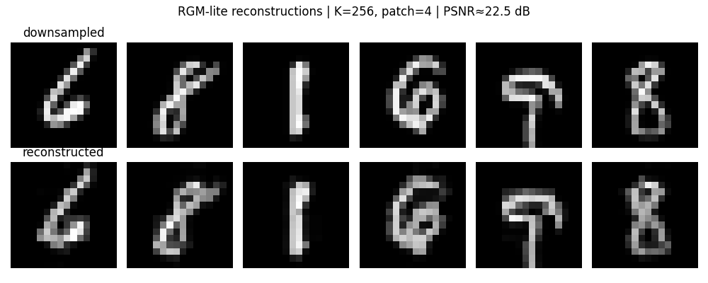
Fig. 9: Proof’s in the puddin’.
The bitrate works out to roughly 0.6 bits per pixel, compared to 8 bpp for raw grayscale. Not a compression scheme you’d actually use, but it gives a sense of how aggressively the model is summarizing.
Exercises for the reader
The model gets decent accuracy on MNIST (as unimpressive as that might seem), but there are a few things that could make it noticeably better without changing the basic approach. I’m sure there are others I haven’t thought of.
- Learn
p(supertoken | class, position)instead ofp(supertoken | class). Right now the model treats all four supertoken positions as interchangeable, which means it can’t distinguish digits that use similar strokes in different arrangements. Expanding the count array from(C, K2)to(C, 4, K2)is all it takes. - Use soft token assignments. Instead of hard-assigning each patch to its nearest centroid, convert distances to weights and propagate the ambiguity. We already marginalize over supertokens during inference, doing the same at the token level is the natural next step. This would also bring it closer to a real RGM.
- Make
psiclass-dependent: learnp(token | supertoken, class)instead ofp(token | supertoken), which would mean that there are more parameters, but use the same counting machinery.
The first one is probably the biggest win for the least effort, while the second one will bring it the closest to the conceptual spirit of the RGM.
Fin
The classifier is about 150 lines of code, the whole program just under 300 lines with comments. No prefab neural networks, no optimization loops. It classifies MNIST digits by counting. A proper RGM would do much more, but the skeleton is there: spatial coarse-graining, hierarchical generative model, and Bayesian inference. I had fun building it. I hope the run-through was valuable.
The code is here if you want to check it on your own time.
1. If you actually know renormalization group theory and I’ve gotten something meaningfully wrong, I’d appreciate hearing about it!
2. You could work with the original 28x28 images, but 28 doesn’t divide evenly by 4, and dealing with remainder pixels adds complexity that isn’t interesting. Downsampling to a power-of-two-friendly size keeps the code simple.
3. You know it’s serious when the capital letters come out to play.